
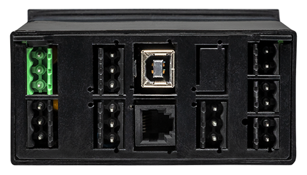
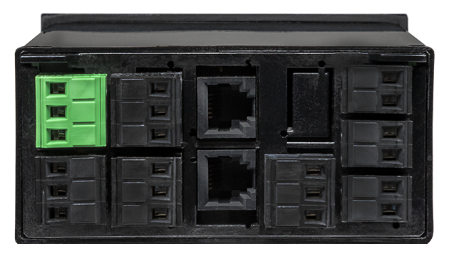
Features
- Times periodic events with width from 1 µs to 199.999 s
- Transmits average time of periodic events with width from 1 µs to 199.999 s
- Resolution to 0.2 µs, rep rated to 250 kHz
- Inputs from NPN or PNP proximity switches, contact closures, digital
logic, magnetic pickups down to 12 mV, or AC inputs up to 250 Vac - Trigger on positive or negative pulse edges
- Wide choice of Plug-in-Play options:
- 2 or 4 relays, mechanical or solid state, for alarm or control (isolated)
- 1 or 2 Analog output, 4-20 mA, 0-20 mA, 0-10V, or -10V to +10V (isolated)
- Communications: Ethernet, WiFi, USB, RS232, RS485 (isolated)
- Extended DPM includes rate and total simultaneously, dynamic up-down
Certificates of Compliance
The Laureate™ 1/8 DIN Digital Panel Meter for A-to-B Time Interval
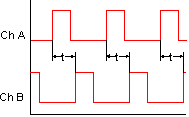
can display pulse width or time delay between individual pulses to a resolution of 0.2 µs. It can also display average pulse width or average time delay between multiple pulses.Time interval is measured between inputs on channels A and B. Timing starts when a pulse is applied to Channel A (selectable positive or negative edge), and ends when a pulse is applied to Channel B (selectable positive or negative edge). In case of a single pulsed signal, the A and B inputs can be tied together. A positive or negative slope may be selected to start timing, and the opposite slope must be selected to stop timing. Timing is achieved by counting 5.5 MHz clock pulses. Multiple integral time intervals are averaged over a gate time which is selectable from 10 ms to 199.99 s and also controls the display update time.
Time interval can be displayed in seconds, milliseconds, or microseconds with 6-digit resolution. In the typical application, time is displayed in milliseconds with 1 µs resolution. For times less than 100 ms, display resolution down to 0.2 µs can be achieved by applying a multiplier of 10, moving the decimal point by one position, and averaging many time intervals.
Highly accurate rate can be displayed by taking the inverse of time. Extensive arithmetic capabilities allow display in engineering units, such as meters/sec. An Extended main board version offers all features of Standard main board plus rate based on 1/time.
The FR dual-channel signal conditioner board accepts inputs from proximity switches with a PNP or NPN output, TTL or CMOS logic, magnetic pickups, contact closures, and other signals from 12 mV to 250 Vac. Jumper selections provide optimum operation for different sensor types and noise conditions. A built-in (isolated) 5, 10, 12, or 24 Vdc excitation supply can power proximity switches and other sensors, and eliminate the need for an external power supply.
Extended DPM includes rate and total simultaneously, dynamic up-down counting, arithmetic functions applicable to channels A & B (A+B, A-B, A/B, AxB, A/B-1), phase angle, power factor, duty cycle, batch control, custom curve linearization.
The Laureate Digital Panel Meter is easily programmed with Laurel’s free Instrument Setup Software, downloadable from our website and compatible with Windows PCs, requiring a data interface board for setup.
All signal conditioner board ranges are factory-calibrated, with calibration factors for each range securely stored in an onboard EEPROM. These factors can be scaled via software to accommodate external shunts, enabling field replacement of signal conditioner boards without necessitating recalibration of the associated digital panel meter. For optimal accuracy, factory recalibration is recommended annually. All Laurel Electronics instruments undergo factory calibration using the industry-leading Fluke calibrators, which are recalibrated yearly and certified traceable to national standards, ensuring the highest level of precision and reliability.
Digital signal filtering modes can be selected to ensure stable readings in electrically noisy environments.
- An unfiltered selection provides true peak and valley readings and aids in control applications.
- A batch average filter selection averages each 16 conversions.
- An adaptive moving average filter selection provides a choice of 8 time constants from 80 ms to 9.6 seconds. When a significant change in signal level occurs, the filter adapts by briefly switching to the shortest time to follow the change, then reverts back to its selected time constant. An Auto setting selects the time constant selection based on signal noise.
Peak and valley values are automatically captured. These may be displayed via a front panel pushbutton command or control signal at the rear connector, or be transmitted as serial data.
Two rear panel control Inputs (CMOS/TTL levels, logic 0 = tied to digital ground, logic 1 = open) or dry contacts that can be set to control / activate 14 meter commands.
An (isolated) 5, 10, 12, or 24 Vdc excitation output is standard to power transducers or two-wire transmitters. Ratiometric operation, which automatically compensates for changes in the applied excitation, is jumper selectable for applications, such as bridges, where the signal to be measured is proportional to the excitation level.
| Display | |
|---|---|
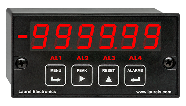
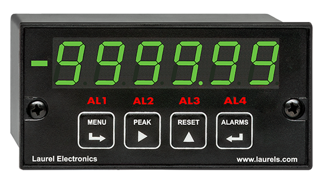
| Readout | 6 LED digits, 7-segment, 14.2 mm (.56"), red or green. |
| Range | -999,999 to +999,999 |
| Indicators | Four LED lamps |
| Inputs | |
| Types | AC, pulses from NPN, PNP transistors, contact closures, magnetic pickups. |
| Signal Ground | Common ground for channels A & B |
| Channel A Freq. | 0 Hz to 1 MHz |
| Channel B Freq. | 0 Hz to 250 kHz |
| Minimum Signal | Nine ranges from (-12 to +12 mV) to (+1.25 to +2.1V). |
| Maximum Signal | 250 Vac |
| Noise Filter | 1 MHz, 30 kHz, 250 Hz (selectable) |
| Recalibration: All ranges are calibrated at the factory. Recalibration is recommended every 12 months. | |
| Time Interval Mode | |
| Timing Start | Channel A pulse, + or - edges |
| Timing Stop | Channel B pulse, + or - edges |
| Periodic Timing Interval | Gate time + 30 ms + 0-2 time intervals |
| Gate Time | Selectable 10 ms to 199.99 s |
| Time Before Zero Output | Selectable 10 ms to 199.99 s |
| Resolution | |
| 0 - 199.999 s | 1 ms |
| 0 - 99.9999 s | 100µs |
| 0 - 9.99999 s | 10 µs |
| 0 - .999999 s | 1 µs |
| 0 - .099999 s | 0.2 µs |
| Accuracy | |
| Time Base | Crystal calibrated to ±2 ppm |
| Span Tempco | ±1 ppm/°C (typ) |
| Long-term Drift | ±5 ppm/year |
| Maximum Signal | |
| Max applied voltage | 600 Vac for 20, 200 and 300 V ranges, 125 Vac for other ranges |
| Overcurrent protection |
25x for 2 mA, 8x for 20 mA, 2.5x for 200 mA, 1x for 5 A |
| Power Supply Boards (one required) | |
| Voltage, standard | 85-264 Vac or 90-300 Vdc |
| Voltage, optional | 12-32 Vac or 10-48 Vdc |
| Frequency | DC or 47-63 Hz |
| Power consumption | 1.2W @ 120 Vac, 1.5W @ 240 Vac, 1.3W @ 10 Vdc, 1.4W @ 20 Vdc, 1.55W @ 30 Vdc, 1.8W @ 40 Vdc, 2.15W @ 48 Vdc (typical, base meter) |
| Power Isolation | 250V rms working, 2.3 kV rms per 1 min test |
| Excitation Output (standard) | |
| 5 Vdc | 5 Vdc ± 5%, 100 mA (jumper selectable) |
| 10 Vdc | 10 Vdc ± 5%, 120 mA (jumper selectable) |
| 12 Vdc | 12 Vdc ± 5%, 100 mA (jumper selectable) |
| 24 Vdc | 24 Vdc ± 5%, 50 mA (jumper selectable) |
| Output Isolation | 50 Vdc from signal ground |
| Analog Output Boards (one optional) | |
| Output levels | 4-20 mA, 0-20 mA, 0-10V, -10 to +10V (jumper selectable) |
| 4-20 mA, 0-20 mA, 0-10V (dual-output option) | |
| Current compliance | 2 mA at 10V ( > 5 kΩ load) |
| Voltage compliance | 12V at 20 mA (< 600 Ω load) |
| Scaling | Zero and full scale adjustable from -99999 to +99999 |
| Resolution | 16 bits (0.0015% of full scale) |
| Isolation | 250V rms working, 2.3 kV rms per 1 min test |
| Relay Output Boards (one optional) | |
| Dual magnetic relays | 2 Form C, 10A max, 440Vac or 125Vdc max, 2500VA or 300W |
| Quad magnetic relays | 4 Form A (NO), 10A max, 440Vac or 125Vdc max, 2500VA or 300W |
| Dual solid state relays | 2 Form A (NO), AC or DC, 0V - 400V, 120Ma, 35Ohms (max at On-State) |
| Quad solid state relays | 4 Form A (NO), AC or DC, 0V - 400V, 120Ma, 35Ohms (max at On-State) |
| Relay commons | Isolated commons for dual relays or each pair of quad relays |
| Relay isolation | 250V rms working, 2.3 kV rms per 1 minute test |
| Relay latching modes | Latching or non-latching |
| Relay active modes | Active on or off, active high or low |
| Hysteresis modes | QA passband mode, split hysteresis, span hysteresis |
| Communication Boards (one optional) | |
| Board selections | RS232, RS485 with dual RJ11 connectors, RS485 with dual RJ45 connectors, USB, Ethernet, USB-to-RS485 gateway, Ethernet-to-RS485 gateway, WiFi with built-in antenna plus USB & RS485, WiFi with external antenna plus USB & RS485 |
| Protocols | Laurel Custom ASCII (serial), Modbus RTU (serial), Modbus TCP (Ethernet or WiFi) |
| Digital addresses | 247 (Modbus), 31 (Laurel ASCII), |
| Isolation | 250V rms working, 2.3 kV rms per 1 min test |
| Environmental | |
| Operating temperature | -40°C to 70°C (-40°F to 158°F) |
| Storage temperature. | -40°C to 85°C (-40°F to 185°F) |
| Relative humidity | 95% at 40°C, non-condensing |
| Protection | NEMA-4X (IP-65) when panel mounted |
| Signal Connections | |
 |
|
| Mechanical | |
| Enclosure | 1/8 DIN, high impact plastic, UL 94V-0, color: black |
| Mounting | 1/8 DIN panel cutout required: 3.622" x 1.772" (92 mm x 45 mm). |
| Dimensions | 4.68" x 2.45" x 5.64" (119 mm x 62 mm x 143 mm) (W x H x D) |
| Maximum panel thickness | 4.5 mm (0.18") |
| Tightening Torque - Connectors | Screw terminal connectors: 5 lb-in (0.56 Nm) |
| Tightening Torque - Pawls | Digital Panel Meter Case Pawls: 5 lb-in (0.56 Nm) |
| Weight of base meter | 210 g (7.4 oz) typical (DPM, counter, timer, 6-digit remote display) |
| Weight of option boards | 30 g (1.0 oz) typical per board (analog output, relay output, communications) |
| General | |
| Programming Methods | Four front panel buttons or via Laurel's free Instrument Setup Software, which runs on a PC under MS Windows. |
| Security | Lockout options include using the front panel buttons, the free Instrument Setup Software, or a hardware jumper. |
| Warranty | 3 years parts & labor |
| Recalibration: All ranges are calibrated at the factory. Recalibration is recommended every 12 months. | |
Free Instrument Setup Software for Series 2 Laureates
|
|
| 1/8 DIN Digital Panel Meters | DIN Rail Transmitters |
Free Downloadable Windows-based Instrument Setup (IS) software (Data Interface Board Required) for use with our programmable Digital Panel Meters, Scale Meters, Counters, Timers, Remote Displays, and Transmitters, are an easy method to set up Laureate 1/8 DIN digital panel meters, counters, timers, remote displays, and DIN-rail transmitters, as explained in the Instrument Setup Software Manual. Laureate 1/8 DIN instruments can also be set up from the front panel, as explained in their respective Owners Manuals. Instrument Setup software is of benefit whether or not the PC is connected to the instrument.
- When the PC is connected to the instrument, Instrument Setup software can retrieve the setup file from the instrument or open a default setup file or previously saved setup file from disk View Setup, then provides graphical user interface (GUI) screens with pull-down menus applicable to input, display, scaling, filtering, alarms, communications, analog output, and front panel lockouts. Fields that are not applicable to the instrument as configured are either left out or grayed out. Clicking on any item will bring up a detailed Help screen for that item. After editing, the setup file can be downloaded, uploaded to the instrument, or saved to a disk. The same setup file can then be downloaded into multiple instruments.
- When the PC is not connected to the instrument, the above GUI screens can be used to set up a virtual instrument. The setup file can then be saved to disk. Switching toView Menu then brings up a screen with the required front panel programming steps. This view can be printed out for use at the instrument site and to serve as a hard copy record.
Download Free Instrument Setup Software
Installation
Set User Account Control (UAC) of MS Windows to "Never notifiy me" so that Instrument Setup Software can create directories. The UAC change screen can be reached as follows:
- Under Windows 7, click on the Windows Start button in the lower left of the desktop and enter "UAC" in the search field.
- Under Windows 8, navigate to Control Panel, then to the "User Accounts and Family Safety" section, and click on "Change User Account Control Settings."
- Under Windows 10, click on the Windows Start button in the lower left of the desktop, then on "Settings", and enter "UAC" in the search field.
- Reboot your computer for the changed UAC setting to take effect.
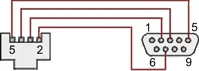
RJ11-to-DB9 cable with rear view of DB9 connector to PC
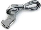
RS232 cable, meter to PC, P/N CBL01
Laureate 1/8 DIN Laureate instruments must be equipped with a serial communications board and be connected to the computer via a serial communications cable. The connection can be via RS232, RS485, USB or Ethernet. Following setup, the serial communications board may be removed from the instrument if desired. The wiring of the RS232 cable is illustrated above with end views of the two connectors.
Laureate LT Series transmitters come standard with a 3-wire serial interface, which can be jumpered for RS232 or RS485.
Laureate LTE Series transmitters come standard with an Ethernet interface.
Meter Setup Screens
Click on any of the reduced screens below for a full-size screen view, then click on the Back button of your browser to return to this page. The screens examples below are for a fully-loaded Series 2 Digital Panel Meter (DPM), which is connected to the PC via RS232. If the meter is a Series 1 meter (pre-2007), this is sensed by the software, and somewhat different screens are brought up. Please see Series 1 setup screens.

Welcome Screen
From the computer desktop, click on Start > Programs > IS2 > IS2. Or click on the IS icon on your desktop. This splash screen will be displayed for three seconds. The software revision number is in the lower right.


Communications Selection Screen
Specify your desired communication protocol and the serial communications bus type, which should match the jumper setup of the instrument. Select None if the PC is not connected to the instrument.

Establish Communications Screen
If you selected RS-232, you will be asked to specify the PC Com Port and Baud Rate, which should match the jumper setup of the instrument. Click on Establish. With the right settings, the Communications Established field will light up in green, and the Meter Type will be recognized. If so, click onMain Menu.

Main Menu Screen
Click on File > Default Setup to retrieve the default setup file from disk for your type of meter. Click on File > Open Setupto retrieve a previously saved setup file from disk or on File > Save Setup to save your edited setup file to disk. Click onDPM > Get Setup to retrieve the setup file from your meter or on DPM > Put Setup to download your edited setup file into the meter.

DPM Input + Display Setup Screen
From the Main Menu, click on View > Setup, then on theInput+Display tab. You can now specify the meter hardware, signal type, display mode, and functions of control inputs A and B. Clicking on any item brings up a pull-down menu with the available choices.

DPM Scaling Setup Screen
Click on the Scaling tab, which provides three scaling methods to relate the signal to the displayed reading: 1) Scale and Offset method, 2) Coordinates of two points method, and 3) Reading Coordinates of Two Points method. The last method uses actual high and low signals, and the computer will prompt you.

DPM Filter Setup Screen
Click on the Filter tab, which allows you to specify the digital filter time constant (if any), the adaptive filter threshold, and whether Peak / Valley values are filtered or unfiltered. As for all setup screens, clicking on the F1 key while an item is highlighted brings up a Help screen for that item, as illustrated.

DPM Relay Alarms Setup Screen
Click on the Relay Alarms tab, which allows you to set up Alarms 1 and 2 for the optional dual relay output board. Clicking on any of the four numeric fields changes these to green and brings up a special field to enter the desired numeric value, which is tied to the displayed reading.

DPM Communications Setup Screen
Click on the Communications tab so set up serial communications. In particular, you can special the Serial Protocol and the meter address if multiple meters are to be addressed on the same serial data line.

DPM Analog Output Setup Screen
Click on the Analog Out tab so set up the optional analog output board. Three output ranges are selectable, the endpoints of which can be tied to user-specified High and Low readings.

DPM Lockouts Setup Screen
Click on the Lockouts tab to check off menu items which will no longer be accessible from the front panel of the meter. This will simplify meter operation and prevent unintended setup changes.
Meter Setup Utilities

DPM Front Panel Setup Screen
As an aid to programming the meter from the front panel when a serial connection is not available, you can return to the Main Menu and click on View > Menu. The required sequence of front panel screens will then be displayed. Click on any step in the sequence for the meaning of each digit, as illustrated for the FILtEr step. For a hardcopy, simply press on Print.

DPM Jumper Setup Screen
Specify your desired communication protocol and the serial communications bus type, which should match the jumper setup of the instrument. Select None if the PC is not connected to the instrument.

DPM Jumper Setup Screens
Click on any of the displayed plug-in boards, and you will be presented with the jumper positions and electrical connections for your selected board. This minimizes the need to refer to the printed manual.

DPM Commands Screen
This page allows you set up external input, serial communications, an analog output proportional to the display (optional), and lockouts for Laureate digital counters. The grayed out area at the top right of the screen applies to Laureate remote displays.


Graphical Output Screens (not available with Ethernet)
From the Main Menu, click on Readings if your PC is connected to the meter. A pull-down menu then offers three choices: List, Plot and Graph.
- List presents the latest readings in a 20-row by 10-column table. Press Pause at any time to freeze the display. This is one method to capture peak readings.
- Plot generates a plot of readings vs. time in seconds. It effectively turns the DPM-PC combination into a printing digital oscilloscope.
- Graph generates a histogram where the horizontal axis is the reading and the vertical axis is the number of occurrences of readings. The display continually resizes itself as the number of readings increases.

DPM Calibration Screens
Click on the Scaling tab, which provides three scalClick on the Scaling tab, which provides three scaling methods to relate the signal to the displayed reading: 1) Scale and Offset method, 2) Coordinates of two points method, and 3) Reading Coordinates of Two Points method. The last method uses actual high and low signals, and the computer will prompt you.

Frequency Meter Calibration Screen
Calibration of the quartz crystal of the Laureate frequency meter requires the input of a known frequency from a calibrator. Apply the frequency, then enter the frequency in Hertz. Calibration will be automatic, with storage of the calibration factor stored in non-volatile memory.
Laureate™ 1/8 DIN Case For Laureate Digital Panel Meters, Counters, Timers & Remote Displays
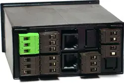
Key Features
- Meets 1/8 DIN Standard.
- Installs from front of panel.
- Short depth behind the panel: only 4" (102 mm) plus connectors.
- Understated 0.157" (4 mm) thick bezel.
- Meets NEMA 4X (IP-65) for high-pressure wawshdon when panel mounted.
- Screw clamps connectors meet VDE / IEC / UL / CSA safety standards.
- Rugged GE Lexan® housing material.
- Safety certified per EN 61010-1.


Dimensions
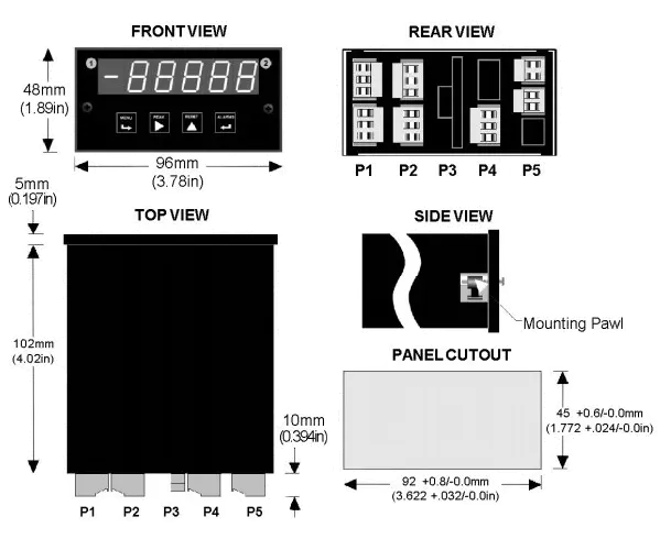
Maximum panel thickness: 4.5 mm (0.18")
Weight of base meter: 210 g (7.4 oz) typical (DPM, counter, timer, 6-digit remote display)
Weight of option boards: 30 g (1.0 oz) typical per board (analog output, relay output, communications)
Tightening Torque - Connectors: Screw terminal connectors: 5 lb-in (0.56 Nm)
Tightening Torque - Pawls: Digital Panel Meter Case Pawls: 5 lb-in (0.56 Nm)
Dimensioned CAD assembly drawings in EPRT, STEP, x_t. dwg, pdf file formats: Laureate-meter-case.zip (zipping prevents browser from opening CAD files as text files).
Panel Mounting
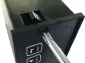 Slide the meter into a 45 x 92 mm 1/8 DIN panel cutout. Ensure that the provided gasket is in place between the front of the panel and the back of the meter bezel.
The meter is secured by two pawls, each held by a screw, as illustrated. Turning each screw counterclockwise extends the pawl outward from the case and behind the panel. Turning each screw clockwise further tightens it against the panel to secure the meter.
Slide the meter into a 45 x 92 mm 1/8 DIN panel cutout. Ensure that the provided gasket is in place between the front of the panel and the back of the meter bezel.
The meter is secured by two pawls, each held by a screw, as illustrated. Turning each screw counterclockwise extends the pawl outward from the case and behind the panel. Turning each screw clockwise further tightens it against the panel to secure the meter.
Turning each screw counterclockwise loosens the pawl and retracts it into its well. This position allows installed meter to be removed from their panel, or new meters to be installed in a panel. Do not remove the screws from their pawls. Doing so would cause the screw and pawl to fall off and likely get lost. Do not overtighten so as not to damage the plastic parts.


| Time Interval Mode for Time Delay | |
|---|---|
|
For periodic pulses applied to A and B channels, time delays can be measured down to 0.2 µs resolution from the rising or falling edge of A to the rising or falling edge of B (selectable). |
| Time Interval Mode for Pulse Width | |
 |
The width of periodic pulses (t1 or t2) can be measured by tying the A and B channels together. As for time delay, readings are averaged over a user-selectable gate time. |
| Timing Process Dynamics with a Panel Meter and Time Interval Meter | |
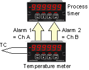 |
The start and stop pulses used for timing can be generated by the dual relay board in a Laureate panel meter or digital counter. For instance, the start and stop pulse edges can be created as temperature passes two alarm setpoints, or temperature cycles in a hysteresis control mode. |
| Rate Based on 1 / Time | |
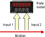 |
The Extended stopwatch meter can be programmed to display highly accurate rate based on elapsed time. A pulse or switch closure can initiate timing, while another pulse or switch closure stops timing. The meter can be programmed with multipliers to display rate in appropriate engineering units, such as meters/sec, for any time duration. |
| Replacing an Oscilloscope with a Laureate Time Interval Meter | |
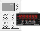 |
An oscilloscope is great for viewing and timing pulses in a lab. However, in fixed installations where digital timing accuracy and control outputs are required, a low-cost Laureate time interval meter will be the instrument of choice. Resolution to 0.2 µs is feasible. |
| Instrumenting a Pulsed Laser System Using Laureate Counters | |
 |
|
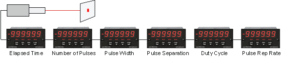
| Some of the many possibilities in instrumenting a pulsed laser system with Laureate dual-channel counters. | |
CAL-Digital
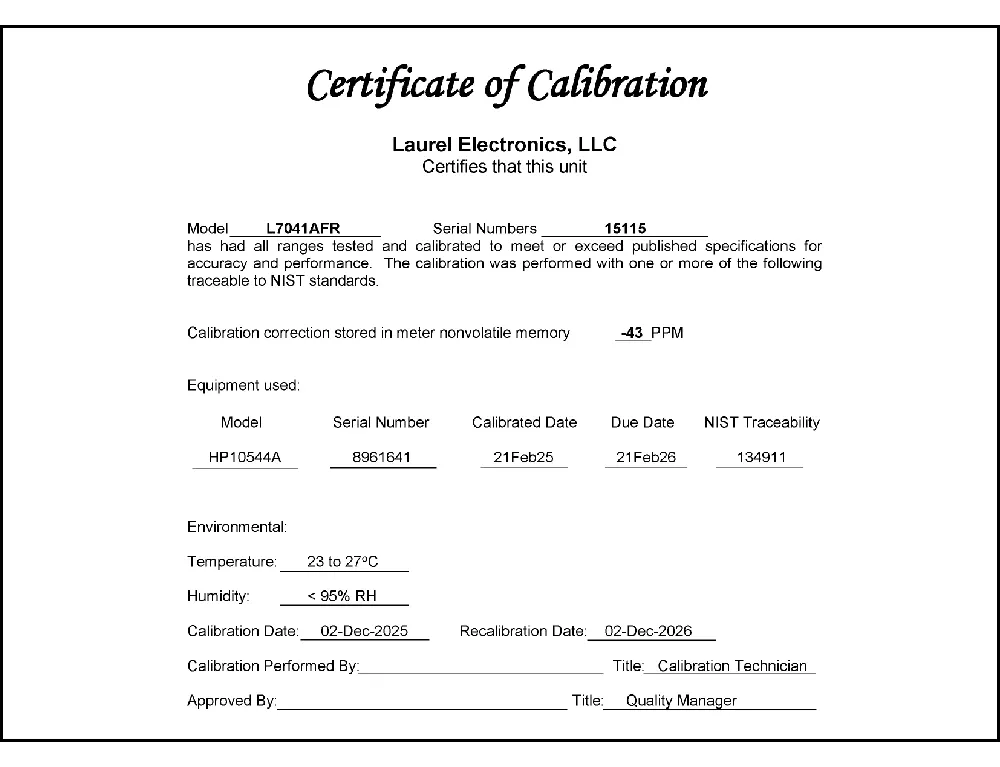
Certificate of Calibration
$65.00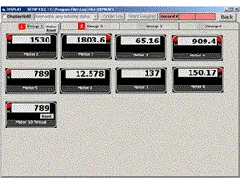
DLS-XLOG2
XLog2 Data logging Software
$495.00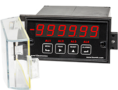
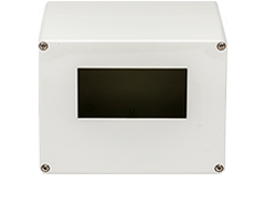
IPC
Splashproof Cover
$55.00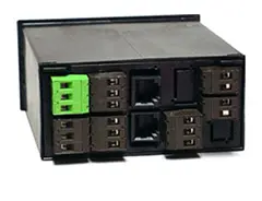

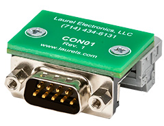
CON01
CON01 Connector
$75.00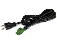
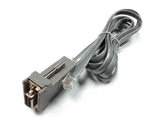
CBL01
RS232 Cable for Meters
$35.00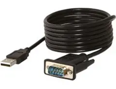
CBL02
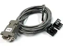
USB-to-RS232 Adapter Cable
$47.00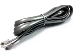
CBL04
RS232 Cable for LT Transmitters
$47.00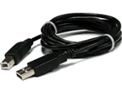
CBL05
USB Data Cable for Meters
$47.00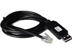
CBL06
USB-to-RS485 Adapter Cable
$47.00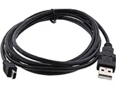
CBL07
USB Programming & Data Cable
$47.00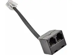
CBL08
RS485 Splitter Cable
$33.00CBL6
6-foot Power Cable
$41.00CBL12
12-foot Power Cable
$47.00Modular Design for Maximum Flexibility at Minimum Cost
All boards are isolated from meter and power grounds. Optional Plug-in-Play boards for communications and control include Ethernet, WiFi, serial communication boards, dual or quad relay boards, and an analog output board. Laureates may be powered from 85-264 Vac or optionally from 12-32 Vac or 10-48 Vdc. The display is available with bright red or green 0.56" (14.2mm) high LED digits. The 1/8 DIN case meets NEMA 4X (IP65) specifications from the front when panel mounted. Any setup functions and front panel keys can be locked out for simplified usage and security. A built-in 5, 10, 12, or 24 Vdc excitation supply can power transducers, eliminating the need for an external power supply. All power and signal connections are via UL / VDE / CSA rated screw clamp plugs.
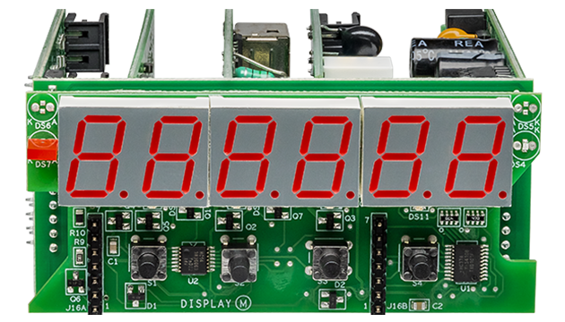
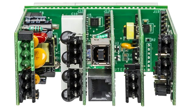
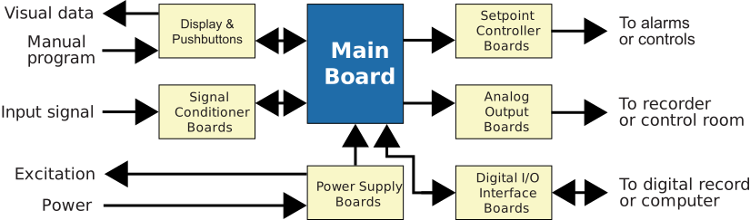
The Laureate™ Series features modular design with up to 7 isolated plug-in boards, applicable to all Laureate 1/8 DIN Digital Panel Meter.
Modular Hardware
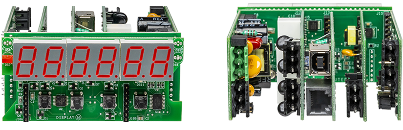
The design of the Laureate™ Series is modular for maximum flexibility at minimum cost. All boards are isolated from meter and power grounds. The base configuration for a digital panel meter or counter consists of a main module (with computer and plug-in display boards), a power supply board, and a signal conditioner board. Optional plug-in-play boards include an isolated setpoint controller board, an isolated analog output board, and an isolated digital interface board. Modular design and a choice of plug-in options allow the Laureate to be customized for a broad range of applications from simple monitoring to control and computer interface. There can be up to five plug-in boards in a 1/8 DIN Laureate.
Connecting Laureate Digital Panel Meter to a Local Area Network (LAN)
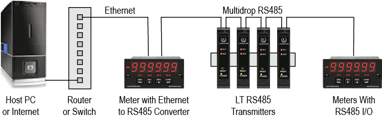
Up to 30 Laureate Digital Panel Meter and/or LT Transmitters can be configured for RS485 and daisy-chained to an LT Transmitter using Laurel’s High Speed Ethernet-to-RS485 converter board for seamless LAN integration. Alternatively, Laurel LTE series Ethernet transmitters can connect directly to a LAN via an Ethernet cable. Setup for both configurations is streamlined using Laurel’s free Instrument Setup Software, which simplifies node discovery and transmitter configuration.
Flexible Communication Options for Digital Panel Meter
The Laureate Digital Panel Meter can be equipped with Laurel communication boards to support various interfaces and protocols. These include serial interfaces with ASCII or Modbus RTU protocols, and Ethernet interfaces with web access, ASCII, or Modbus TCP/IP protocols, ensuring versatile connectivity for your commercial applications.
Understanding the Laureate™ Digital Panel Meter for Time Interval of Periodic Events
The Laureate™ 1/8 DIN Digital Panel Meter for A-to-B Time Interval can display pulse width or time delay between individual pulses to a resolution of 0.2 µs, or the average pulse width or average time delay across multiple pulses. Timing starts when a pulse is applied to Channel A (selectable positive or negative edge) and ends when a pulse is applied to Channel B (selectable positive or negative edge). For a single pulsed signal, A and B inputs can be tied together, with a positive or negative slope starting timing and the opposite slope stopping it.
Timing Technique and Resolution
Timing is achieved by counting 5.5 MHz clock pulses. Multiple integral time intervals are averaged over a gate time selectable from 10 ms to 199.99 s, which also controls display update time. Resolution scales by range: 1 ms for 0-199.999 s, 100 µs for 0-99.9999 s, 10 µs for 0-9.99999 s, 1 µs for 0-.999999 s, and 0.2 µs for 0-.099999 s. For times under 100 ms, display resolution down to 0.2 µs can be achieved by applying a ×10 multiplier, shifting the decimal point one position, and averaging many time intervals.
Rate From Time and Signal Specifications
Highly accurate rate can be displayed by taking the inverse of time, with arithmetic capability for engineering units like meters/sec — this requires the Extended main board. Periodic timing interval equals gate time plus 30 ms plus 0-2 time intervals; Time Before Zero Output is separately selectable from 10 ms to 199.99 s. Maximum applied voltage is 600 Vac for the 20V/200V/300V ranges, 125 Vac for other ranges; overcurrent protection is 25x for 2 mA, 8x for 20 mA, 2.5x for 200 mA, 1x for 5A.
Real-World Applications
- Time Interval Mode for Time Delay — for periodic pulses on A and B channels, time delays are measured to 0.2 µs resolution from the rising or falling edge of A to the rising or falling edge of B.
- Time Interval Mode for Pulse Width — pulse width is measured by tying A and B channels together, with readings averaged over a user-selectable gate time.
- Timing Process Dynamics — start and stop pulses generated by the dual relay board in a Laureate panel meter or digital counter, such as pulse edges created as temperature passes two alarm setpoints or cycles in hysteresis control.
- Rate Based on 1/Time — a pulse or switch closure initiates timing, another stops it, with multipliers programmed to display rate in engineering units like meters/sec for any duration.
- Replacing an Oscilloscope — for fixed installations needing digital timing accuracy and control outputs, 0.2 µs resolution is feasible at low cost.
- Instrumenting a Pulsed Laser System — one of many possibilities using Laureate dual-channel counters.
Factory-Calibrated Accuracy
All signal conditioner board ranges are factory-calibrated, with calibration factors stored in EEPROM. Field replacement of the signal conditioner board doesn't require recalibrating the meter. Factory recalibration is recommended annually.
Where Time Interval Digital Panel Meters Are Used
- Laser Pulse Characterization — pulse width, separation, and repetition rate measurement.
- Delay & Propagation Timing — time-delay measurement between correlated events on separate channels.
- Fixed-Installation Test Bench Replacement — permanent digital timing with control outputs.
- Process Dwell Timing — relay-triggered interval measurement for temperature or process cycling.
- PWM & Duty Cycle Verification — pulse width timing via tied A-B channel configuration.
- High-Speed Component Response Testing — microsecond-resolution delay measurement.
- Rate-From-Time Velocity Applications — speed calculation from timed intervals between two trigger points.
Time Interval Digital Panel Meter Frequently Asked Questions
Why does the meter's resolution improve as the measured time range gets shorter (1 ms at the top range down to 0.2 µs at the bottom)?
The meter's underlying timing mechanism is documented as counting a fixed 5.5 MHz clock — since the meter's six-digit display has a fixed number of digits to represent the reading, a shorter maximum range lets each display digit represent a proportionally finer absolute time increment, which is why the documented resolution scales finer as the selected range shrinks.
How does the ×10 multiplier trick actually extend resolution below 100 ms without the meter's underlying clock rate changing?
Documented technique specifically describes applying a ×10 multiplier and shifting the decimal point one position while averaging many time intervals — this doesn't change the meter's fundamental clock-counting resolution, but combines display scaling with intentional averaging across multiple measured intervals to extract finer effective resolution than a single raw reading would show.
Does averaging multiple time intervals over a longer gate time trade off measurement speed for improved reading stability?
Yes — a longer gate time allows more individual time intervals to be averaged into each displayed reading, generally smoothing out interval-to-interval variation, but also means the display updates less frequently; this is the same general responsiveness-versus-stability tradeoff documented across other Laureate counter modes using gate time.
Why does the "Rate Based on 1/Time" mode specifically require the Extended main board rather than being available on the Standard board?
Documented capability specifically distinguishes the Extended main board as offering additional programmable functions beyond the Standard board, including the arithmetic processing (taking the inverse of time and applying multipliers to reach engineering units) that this rate-display mode depends on — the Standard board's documented feature set doesn't include this additional computation layer.
Does tying Channels A and B together for pulse-width measurement limit the meter to only positive-going pulses, or can it measure negative pulses too?
Documented setup specifically describes selecting a positive or negative slope to start timing, with the opposite slope required to stop timing — this framing applies symmetrically regardless of whether the pulse itself is a positive-going or negative-going pulse, since what matters is which edge direction is configured as the start trigger versus the stop trigger.
In the timing process dynamics application, does the relay board need to be a specific type, or can any Laureate relay-equipped instrument generate the start/stop pulses?
Documented description specifically references "a Laureate panel meter or digital counter" equipped with the dual relay board as the source of start and stop pulses, without restricting this to a specific relay board sub-type — any Laureate instrument with relay outputs configured to change state at the desired trigger conditions (such as two temperature alarm setpoints) can serve this role.
Does the documented "0-2 time intervals" component of the periodic timing interval formula mean up to two complete measurement cycles could be effectively wasted waiting for the next valid interval?
Yes, in the worst case — this documented uncertainty term reflects that after the gate time and fixed 30 ms overhead elapse, the meter may need to wait for the next one or two signal periods to complete a valid measurement before returning a reading, meaning actual response time can vary by up to roughly two signal periods depending on where in the input signal's cycle the gate time happens to end.
Can this meter genuinely substitute for an oscilloscope in every application, or only specific ones?
Only specific ones — documented positioning specifically frames this as the better choice for fixed installations needing digital timing accuracy and control outputs, not as a general oscilloscope replacement; an oscilloscope remains necessary for actually viewing waveform shape, which this meter's numeric timing display doesn't provide.
Does the maximum applied voltage rating (600 Vac vs. 125 Vac depending on range) mean the meter's own timing signal is expected to be that high, or is this a separate protection spec?
This is documented as a protection specification rather than the meter's normal working signal level — timing pulses used for time interval measurement are typically low-level logic or sensor signals, and the 600 Vac / 125 Vac figures describe the input circuitry's rated tolerance against an accidental fault voltage on that range, not the intended operating voltage of a genuine timing signal.
Can the overcurrent protection multipliers (25x for 2 mA, down to 1x for 5A) be interpreted the same way regardless of which range is selected for a given application?
Yes, in the sense that each multiplier is documented relative to its own range's full-scale current — the lower-current ranges carry proportionally more overcurrent headroom because an overcurrent event relative to a small full-scale rating is still a modest absolute current, while the 5A range's 1x rating reflects that its full-scale current is already substantial, leaving comparatively little additional margin before the protection circuitry's own limits are reached.
Timing Jitter & Statistical Averaging Questions From the Field
Does averaging a genuinely large number of timing samples always keep reducing measurement error proportionally, or does the benefit eventually taper off?
Documented analysis of time-of-arrival estimation specifically shows diminishing but real returns — averaging over 100 samples was documented as reducing estimated error from roughly 0.5 of a unit interval down to about 0.06, a substantial but non-linear improvement; the underlying statistical principle is that averaging reduces random error roughly with the square root of the sample count, meaning each additional doubling of samples yields a progressively smaller marginal improvement.
Does the specific statistical distribution of timing jitter (uniform versus Gaussian) change whether averaging is an effective error-reduction strategy?
Not fundamentally — documented simulation results specifically found that averaging remained effective at reducing time-of-arrival estimation error under both a uniform jitter distribution assumption and a more realistic Gaussian jitter distribution, indicating averaging is a broadly applicable technique across different underlying jitter statistics rather than being valid only for one specific distribution shape.
Why do documented jitter-measurement best practices specifically recommend against measuring individual timing samples in isolation?
Documented guidance specifically explains that jitter varies randomly, or with a random component, meaning individual measurements are typically of little standalone value — the documented recommendation is analyzing jitter statistically using tools like histograms across many measurements, extracting parameters like standard deviation and peak values, rather than drawing conclusions from any single measured interval.
Does a longer measurement record (more samples collected) genuinely improve the statistical confidence in a jitter or timing measurement, or is sampling rate what matters more?
Both matter, but for different reasons — documented guidance specifically recommends selecting a relatively large record length specifically so a significant population of jitter data can be captured for statistical analysis, while separately recommending the highest available sampling rate specifically to minimize interpolation error in resolving each individual edge; record length and sampling rate address two genuinely different sources of measurement uncertainty.
Can averaging repeated timing measurements introduce its own distortion, or is it a purely beneficial technique?
It can introduce distortion under some conditions — documented analysis specifically notes that when the underlying signals being averaged contain jitter, the averaged result can be distorted, with higher-frequency content in the result attenuated more than the rest, often visible as artificially slower-looking rising edges in the averaged waveform; averaging isn't a purely beneficial technique without any tradeoffs.
Does re-triggering a time-interval measurement immediately after each reading, without any dead time, generally improve or degrade measurement quality?
Documented technical analysis specifically notes that re-triggering a time-interval measurement typically requires a meaningful dead time between successive measurements, particularly when time interpolation techniques are used to achieve finer-than-clock-period resolution — attempting to eliminate that dead time entirely is documented as a practical limitation rather than a straightforward improvement.
Is there a documented, standard set of statistical parameters typically reported from a batch of repeated timing measurements?
Yes — documented convention specifically reports the count of periods or intervals evaluated, the highest observed jitter value over the measurement window, and the standard deviation of all measured values across that window as the standard statistical summary, often supplemented by histogram or time-versus-time plots for deeper analysis.
Does disabling waveform or reading averaging ever improve, rather than degrade, the accuracy of a specific timing or jitter measurement?
Yes, in specific documented cases — guidance for setting up accurate jitter measurements specifically recommends disabling waveform averaging as one of several steps to reduce measurement error, since the goal in that specific context is to capture and characterize the genuine, unaveraged variation present in the signal rather than smoothing it away before analysis.
